Knots based on dissulfide and ion bonds
Usually, the term "knotted protein" refers to a situation, when the backbone of the protein forms a knot after appropriate chain closure. The choice of the backbone is well justified, as the backbone is composed of strong, covalent bonds, joining the carbon and nitrogen atoms. However, some residues may be also joined non-sequentially, by disulfide bonds, posttranslational amide bonds, or even as a concatenation of the side groups (see Fig. 1). The existence of such bonds results in inter-protein covalent loops, which may in principle be as well knotted. Therefore, the description of protein’s topology requires first the determination of the interaction taken into account.
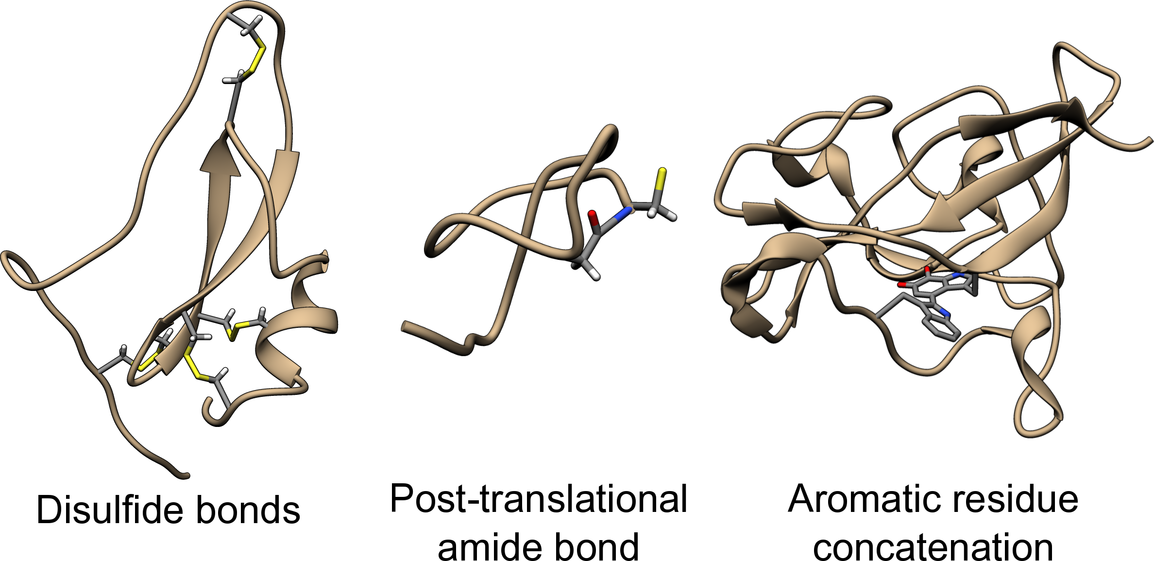
Fig 1. Exemplary protein structures with various covalent bond between non-sequential residues. The disulfide bond (within hydrolase inhibitor with PDB code 2LFK), posttranslational amide bond closing the loop (within replication inhibitor with PDB code 1RPB) and concatenation of aromatic side chains (within oxidoreductase with PDB code 3C75). The atoms of joined residues were shown and colored.
The KnotProt database allows the user to decide, which interactions are the most important to the user’s needs. In particular, when classifying the protein, the KnotProt database extracts all the loops, which may be built with connection of non-consecutive residues by covalent bridges (disulfide etc.), bridges via ions or by connection of the chain termini. The different kind of interactions used in KnotProt are presented in Fig. 2. In particular, when choosing only connection of the termini (probabilistic), the set of knotted protein loops is equal to the standard set of knotted proteins (the default option).

Fig 2. Schematic presentation of three types of interaction included in KnotProt database.
The existence of inter-protein interactions within a knotted protein leads to the existence of knotted loops, closed e.g. by the well-defined interaction via ion. It may happen, however, that the protein has an unknotted backbone, but one may find a covalent, or ion-based loop, which is knotted. This situation is schematically shown in Fig. 3.
By using the filters in the search tab, the user may obtain the proteins with the desired topological properties. On the other hand, the user may also find out, which proteins are unknotted when taking into account given set of bonds (by applying the filters and selecting the "unknot" icon). In particular, one may see, that no loop identified within so-called "cysteine knot" motif is knotted. In fact, the cysteine knot motif can be continuously transformed into (and hence is topologically equivalent to) a simple, unknotted graph, called by the mathematicians a complete graph with 4 vertices - the K4. The treatement of cysteine knot in KnotProt is described here.
The knotoid types that are obtained from the various projections are determined by knotoid invariants. In this work we use the Turaev loop bracket polynomial [1,3] since we use planar knotoids in our analysis. In order to shorten the computational time of the Turaev loop bracket, a variation of the KMT algorithm is applied to the chain. More precisely, the algorithm is applied once the projection plane has been chosen and the two infinite lines through the endpoints are introduced. At each step the algorithm is applied with respect to the two infinite lines.
Fig 3. The schematic presentation of unknotted protein with knotted, covalent loop. The protein backbone is presented in black, the covalent bridges in orange. The knotted loop is highlighted in red.
For a protein with knotted loops formed by covalent or ion-based interactions, the result page is similar to the result page of regular knotted proteins. Including the matrix fingerprint and the structure presentation. There are, however, two main differences, determining the construction of the page:
- There may be more than one knotted loop in a protein;
- The knotted loop follows non-sequential residues, in particular, some intervals may be followed from N- to C- terminus, but some in the opposite direction.
All the knotted loops are stored in one table, with one row corresponding to each knotted loop. Apart from the knot type and miniature of knot scheme, each row contains the key, branching residues, which connection forms the loop. These are either the cysteines, or the residues interacting via ion, or the terminal residues (in case of chain closure). As the disulfide bridges are by far the most common interaction used to form such loops, the non-disulfide connection (e.g. ion-based, chain closure) are given in bold. The type of the loop is given explicitly in the last column and indicated as the background of the row - orange for deterministic loop, green for ion-based, blue for probabilistic (Fig. 5).
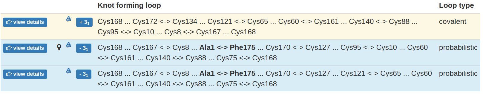
Fig 5. The exemplary table with all the knotted loops identified. Each row contains information about one knotted loop. In particular, it contains the knot type, branching residues forming the loop and the loop type. The loop type is also indicated by the row background color.
To visualize the loop on the structure, the user may click the view details button. This will change the presentation of the protein in JSmol viewer, with the loop indicated in red and branching residues in violet. The connections between residues are shown as red, straight cylinders, including the chain closure or connection via ions. Note that, as in principle, the chain termini can be located further in space, such a connection can be seen as an unnaturally long bond (Fig. 6)
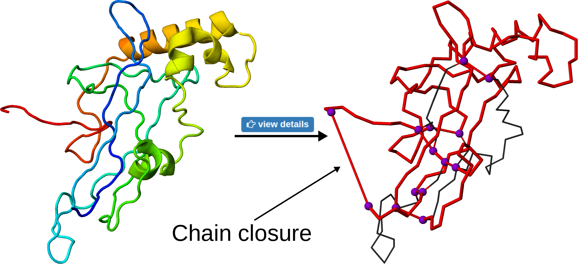
Fig 6. The effect of the "view details" button on the structure. The knotted loop is shown in red, the violet beads denoting the branching residues. The long, straight cylinders denote either termini connection or interactions via ions.
Clicking the view details button affects also the content of the row with structural details placed above the table with the knotted loops. In particular, it shows the details corresponding to the chosen loop (Fig. 7).
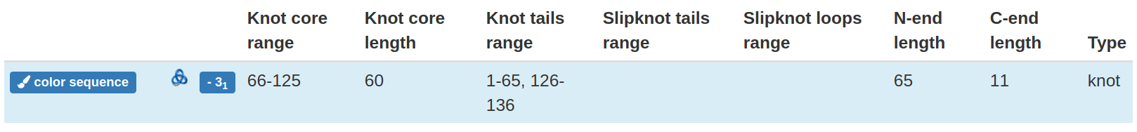
Fig 7. The structural detail of the knotted loop. The content of the row depends on the actually shown loop and is changed by clicking appropriate "view details" button.
To facilitate the understanding of the chain parts used to form a knotted loop, the user may click the color sequence button, which colors each chain interval in the sequence (below the loop table) with a different color. The same colors are used in the JSmol structure presentation (Fig. 8).

Fig 8. The effect of the "color sequence" button on the structure. Each continuous structure interval is colored differently. At the same time, the sequence is colored in such a way to match the structure.
If the user wants to perform deeper analysis using own tools, the coordinates of the loop forming atoms, the result of knot analysis and the figures may be downloaded by clicking the download button.