Search and browse database
There are three main options a user can choose from to view or analyze data:
- Browse database which lists all structures currently deposited in the database; all these structures are also hyperlinked to other databases
- Search and filter database which provides classification of proteins according to their topological, biological, sequential, and geometrical properties
- Process my structure which allows users to upload new polymer-like structures and analyze their topology, or analyze time evolution of entangled structures.
These options are summarized below. Apart from the above options a user can also search proteins according to their PDB code and chain notation. Each option finally will lead the user to:
- Single protein data presentation
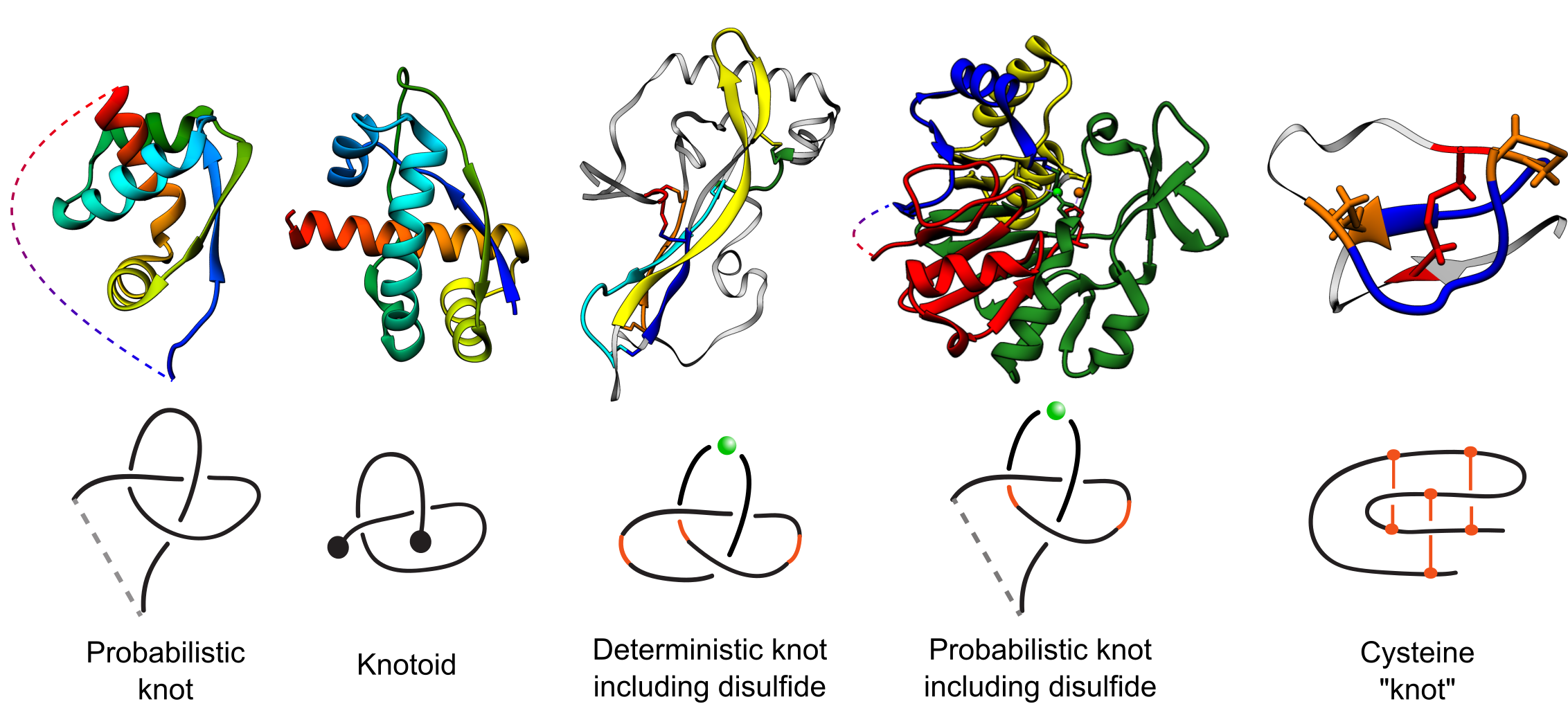
Fig. 1 Types of entanglements identified by the KnotProt 2.0 with exemplary structures. The PDB codes of the structures (left to right): 2efv, 2rh3, 1aoc, 2p4z, 2ml7. The structures are colored blue to red. The light grey, thin parts of the chain are the parts not building the motif. In case of cysteine "knot", the loop-forming bridges are marked orange, while the piercing bridge is marked red.
This option includes all protein chains deposited in the KnotProt database with knots and knotoids formed only based on protein backbone. They can be browsed in three different ways. The default screen presents a list of proteins with their PDB code (together with the chain number specified), the topological notation, and the title used in the PDB header. Proteins with incomplete chains are denoted by an additional symbol of a broken chain element. Another option is to browse a list of names together with miniature figures of knotting fingerprints – this enables users to quickly identify some particular shape of matrix diagram. The third possibility is to browse a list of raw data, which is suitable for independent analysis. Upon choosing one of the listed proteins, the full information about it is presented as described in the section Single protein data presentation.
The filters are located on the top of the page and include:
- Non-redundant proteins or All proteins
- (This option changes the content of all available data on this given website.)
Various entangled structures shown in the Fig. 1 can be filtered by choosing:
- Probabilistic - knots and knotoids formed by protein backbone closed by probabilistic approach. Knots and Knotoids (NEW) are shown in separate tabs. Fig. 2 shows content of the website for the choice "Probabilistic" and "Knotoids".
- Cysteine/ion probabilistic (NEW) - knots formed based on cysteine and ion bridges together with protein backbone closed by probabilistic method (this option is shown in Fig. 3 – left panel)
- Cysteine/ion deterministic (NEW) - knots formed based on cysteine and ion bridges together with protein backbone (this option is shown in Fig. 3 – right panel)
After selecting topological types of interest, user has to click the "Filter" button to display all of the structures matching the criteria chosen.
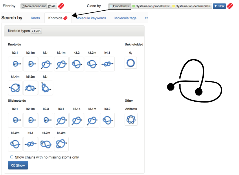
Fig. 2 The default view of the Filter chosen as "Non-redundant" and closed by "Probabilistic" method and Search by Knotoids tab.
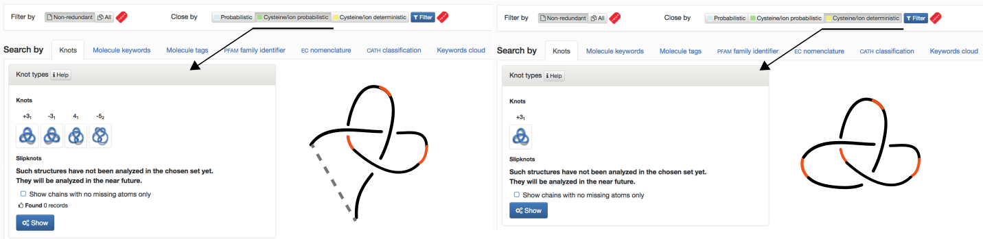
Fig. 3 The default view of the Filter chosen as "Non-redundant" and closed by "Cysteine/Ion probabilistic" (left panel), "Cysteine/Ion deterministic" (right panel) and Search by Knots tab.
A user can search the database in various ways. First, the user can choose between Knots and Knotoids. In the default screen for each of these types the following options can be chosen:
- Knots/Knotoids types: contain four subclassifications: based on a type of knot/knotoid, a type of slipknot/slipknotoid, a list “Other” of proteins with knots/knotoids which must be artefacts (arising from broken protein main chains), and a list “Unknot” of all unknotted (and not containing any knotted subchains) proteins in the PDB
- Fingerprint: classification (separately for knots, knotoids and slipknots,) of proteins according to their knot notation (knotting fingerprint), such as K523131, S3141, etc. In the case of Knotoids only major types of knotoids are shown, however all identified knotoids are listed in raw data which are available for download.
- Knot length and Knot/slipknot depth: knots and slipknots are grouped according to the length of the knot core, as well as the length of the N-terminal and C-terminal tails; those lengths are used to classify knots as shallow or deep (for tails shorter or longer than 10 amino acids respectively).
- NOTE: For knots defined with disulfide bonds or ions taken into account only the knot type is presented. Note that these knots are formed by subchains of protein backbone which may not follow aminoacids’ enumeration. In this case the fingerprint shows the core of the knot.
Moreover several other classifications can be chosen, according to: Molecule keywords, Molecule tags (based on the classification from the pdb website), pfam family identifier, ec nomenclature (numerical classification for enzymes based on the chemical reactions they catalyze), cath classification (which includes class, architecture, and topology), and Keywords cloud. We believe that, based on these classifications, this database will provide the opportunity for other researchers to make new, deep discoveries.
A user can analyze three types of entanglement: knots, slipknots and knotoids, all based on the protein backbone.
A user can upload and analyze two types of data:
- a single structure
- the whole set of structures (e.g. a folding or unfolding trajectory). This option is available only for knots and slipknots.
The data can be submitted either
in the PDB format or in a simplified "x-y-z" format (containing only Cartesian coordinates of atoms, which enables users to analyze arbitrary polymers or open chains).
In the case of a single structure, when knots or slipknots or knotoids are detected by KnotProt 2.0, the relevant knotting fingerprint is constructed. In the case of a trajectory, an xtc format (typical for Gromacs software) can also be uploaded (with a gro or pdb file).
To detect knotting in an open chain, a user can choose:
- probabilistic approach
- direct closure, i.e. connecting two termini by a line segment (for more details see section “Knot detection”). It is also possible to determine a knot type associated to any subchain of the whole chain - in this case a user provides the numbers of two atoms, which are then regarded as the beginning and the end of a subchain.
After selecting a particular protein from the database (e.g. after browsing or searching the database, as described in the next section) users can view all information about it in the following screens:
- Knotting data - the main part of this screen is shown in Fig. 4; it contains the matrix diagram (knotting fingerprint) of a protein (top left), JSmol graphic representation of the protein (top right), a table listing all knots found in subchains of a protein (and detailed information about their lengths, depths, chirality, etc.), and the sequence representation of the protein with knot and slipknot elements (knot core, knot and slipknot tails and loops, etc.) highlighted in colors (bottom). The matrix diagram is interactive: after choosing a knot type (if more than one knot type is detected) from the table, the data corresponding to this knot is shown in the diagram. By default the data corresponding to the knot formed by the whole chain (for knotted proteins), or the most complicated slipknot (for proteins with slipknots) is shown in the diagram.
- Detailed topology (knotoids) - he main part of this screen is shown in Fig. 5; it contains two types of visulization of the topology of analyzed protein:
- Whole chain analysis - projection globes/maps that present the data for the global topology, details are explained here
- Subchain analysis - fingerprint matrices that provide information about the local topology of the chain (details are explained here ). The matrix diagram (knotoid fingerprint) of a protein (top left), JSmol graphic representation of the protein (top right), a table listing all knotoids found in subchains of a protein (and detailed information about their lengths, depths, chirality, etc.), and the sequence representation of the protein with knotoids and slipknotoids elements highlighted in colors (bottom). The matrix diagram is interactive: after choosing a knot type (if more than one knotoid type is detected) from the table, the data corresponding to this knotoid is shown in the diagram. By default the data corresponding to the knotoid formed by the whole chain (for knotted proteins), or the most complicated slipknotoid (for proteins with slipknots) is shown in the diagram.
- Note that a table below the matrix diagram does not list all locations and types of knotoids since some knotoids have very small knotoid core. However, all knotoids and their positions can be found in Download option (details can be found here ).
- Chain information summary - this screen collects basic biological information about the protein: its size, molecule tags and keys, source organism, Enzyme Classification (EC), the number of missing residues, PFAM annotations, etc.; hyperlinks to the PDB, PubMed, PFAM and DOI (if available) are also included.
- Similar chains (by sequence) - provides two lists: the PDB codes of other chains deposited in the KnotProt database with at least 40% sequence similarity, and the PDB codes of other chains (from the full PDB, but not included in the KnotProt) with at least 40% sequence similarity (those proteins should have sequences nearly identical to those deposited in the KnotProt)
- Similar chains (by structures) - lists PDB codes with the same super family or topology or homology, as defined by the CATH database.
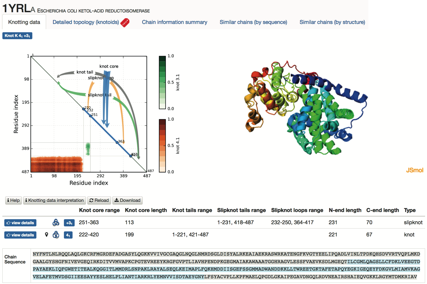
Fig. 4 An example of data presentation for a knotted protein 1yrl in the KnotProt. In this example the analyzed polypeptide chain of E. coli ketol-acid reductoisomerase reveals that the entire polypeptide chain forms a 41 knot, and has a subchain forming a 31 knot. Diagram in top left: knotting fingerprint revealing the positions of subchains forming 41 and 31 knots. Top right: graphical representation of protein in JSmol. Table in the middle: detailed data about knots and slipknots formed by backbone subchains. Bottom: sequence representation with the knot core and knot tails highlighted in various colors.
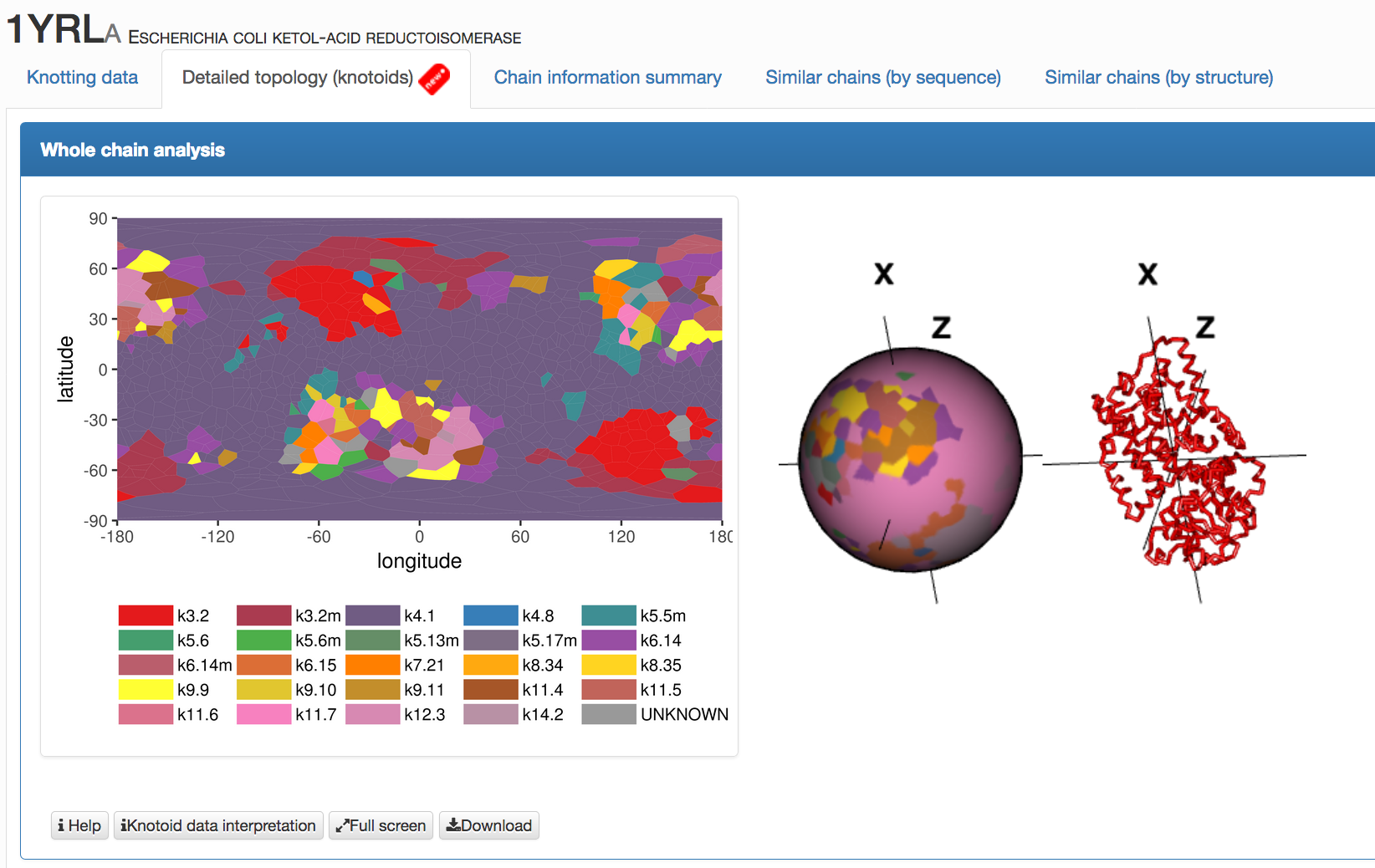
Fig. 5 An example of data presentation for a knotoid formed by protein 1yrl in the KnotProt 2.0. Each point in the map and the projection globe (interactive and colored in the same way as the map) represents the global topology of a knotoid, which is determined by the projection along direction represented by this point.
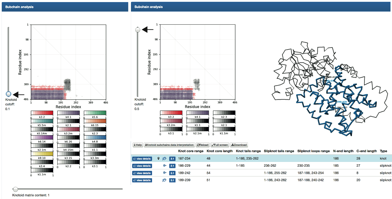
Fig. 6
An example of data presentation for a knotoid formed by protein 1yrl in the KnotProt 2.0. The cursor in the left side of the matrix can be used to show knotoids with lower probability. Left panel shows all identified knotoids with probability as low as 0.1. The right panel shows identified knotoids based on the cutoff used to identify knots. The table below the matrix shows some identified knotoids.